The key is to specify a subgroup size so that significant shifts are detected with high probability and that insignificant shifts are unlikely to produce a signal.
Click here for Part II of this article
The purpose of control charts is to detect significant process changes when they occur. In general, charts that display averages of data/measurements (X-bar charts) are more useful than charts of individual data points or measurements. Charts of individuals are not nearly as sensitive as charts of averages at detecting process changes quickly. X-bar charts are far superior at detecting process shifts in a timely manner, and the subgroup size is a crucial element in ensuring that appropriate chart signals are produced.
WinSPC Means Lower Costs and Higher Quality
WinSPC is software to help manufacturers create the highest quality product for the lowest possible cost. You can learn more here.
Often, the subgroup size is selected without much thought. A subgroup size of 5 seems to be a common choice. If the subgroup size is not large enough, then meaningful process shifts may go undetected. On the other hand, if the subgroup size is too large, then chart signals may be produced from insignificant process shifts. The key is to specify a subgroup size so that significant shifts (from a practical perspective) are detected with high probability and that insignificant shifts are unlikely to produce a signal.
To understand the concept, it is useful to review the impact that averaging data has on variation. The graphic below compares the distribution of individual values with the distributions of averages of various subgroup sizes.
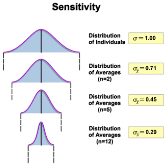
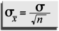
We see that as the subgroup size increases, the standard deviation of the distribution of averages decreases. Specifically, the relationship below relates the standard deviation of averages to the standard deviation of individuals and the subgroup size:
On an x-bar control chart, this idea is reflected by control limits getting tighter as the subgroup size increases.
Now, consider a process that is stable and under statistical control. This curve is represented by the blue curve on the graphic below. Suppose we desire that if the process average shifts by a specified amount (such that it is represented by the red curve below), we would want to obtain a chart signal with very high probability.
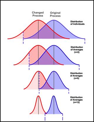
The question is, how likely is it that we will detect the process shift, if in fact the process shifts from the blue curve to the red curve? We consider this question for the 4 cases shown in the above graphic.
In the top set of distributions, we are working with individuals. The control limits for the blue process are represented by the dashed vertical lines. Following the process shift, we will sample from the red curve. Note that most of the red curve still falls inside the control limits for the blue curve. This means that we are very unlikely to see a signal on our chart for the shift indicated.
Now consider the second set of distributions. They represent the case where we are using an x-bar chart with subgroup size = 2. A shift of the same size is shown. Here, the process curves are tighter since they represent averages (with n = 2). While things are better than the first case, there is still a significant overlap between these distributions and it is still not very likely that we will detect the shift quickly.
The case with n = 5 (the third case) is better yet, but still not good enough. We want to be able to detect the shift with high probability.
Finally, with n = 12 (the last case), we see that for the same size shift, the two distributions are practically separate. In other words, if the shift occurs, our next subgroup average will come from the red curve and it will almost certainly be outside of the control limits (based on the blue curve).
Although the above graphics allow us to understand how subgroup size affects chart sensitivity (the ability to detect desired process changes), a formula is typically used to compute the necessary subgroup size for a given application. The subgroup size is a function of the desired sensitivity, the process standard deviation, and the willingness to tolerate type II errors (where the process shifts but the chart fails to detect the shift). The formula is:
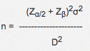
where
n = subgroup size required
Ζ α/2 = the number of standard deviations above zero on the standard normal distribution such that the area in the tail of the distribution is α/2 (α is the type I error probability and is typically 0.0027 for control chart applications. In this case, Ζ 0.00135 =3).
Ζ β = the number of standard deviations above zero on the standard normal distribution such that the area in the tail of the distribution is β (β is the type II error probability).
σ = the standard deviation of the characteristic being charted.
D = the difference we are trying to detect.
View a further discussion on this formula and its application: Click here for Part II of this article.
Steven Wachs, Principal Statistician
Integral Concepts, Inc.
Integral Concepts provides consulting services and training in the application of quantitative methods to understand, predict, and optimize product designs, manufacturing operations, and product reliability. www.integral-concepts.com
Download the white paper on how to jump-start a “mini” Six Sigma Quality program on a budget